
Introduction
During this
semester, you will become very familiar with ordinary differential equations,
as the use of Newton's second law to analyze problems almost always produces
second time derivatives of position vectors. We spend a great deal
of time studying simple problems in depth mostly because of their transparency
- we can readily see and understand how a simple system evolves in time.
By the same token, it is important to realize that very few differential
equations that come from "real world" problems can be solved explicitly,
and often it is necessary to resort to numerical integration for their
solutions. Euler's method is the most basic integration technique
that we use in this class, and as is often the case in numerical methods,
the jump from this simple method to more complex methods is one of technical
sophistication, not conception.
This tutorial is intended for those
with minimal background in spreadsheet use, so if you have experience you
may want to skim the spreadsheet intro parts and pay attention to the later
detailed parts. Also, when you are done with this tutorial, please
email the authors with your response
(see the very bottom of this page).
![]()
Theory
In general, the equation of motion
for a single degree of freedom system can be written as the scalar equation:
So then, if we want to iterate one step forward in time, given the values of v(t1) and x(t1), we would simply substitute in the area of the rectangle for the real integral and get:
![]()
Application
Part of the first
activity assignment involves solving, by Euler's method, the simple
pendulum equation derived in class:
![]()
The Excel Spreadsheet - Integrating the Equation
Spreadsheets are fairly simple to use if you keep in mind that there are three main types of data structures that can be entered into any one cell. If you always remember to check what type of structure each cell contains, you will minimize your chances of frustration. The first type of data is text - ie: you type in a column heading that reminds you what is going to go in that column, or you put your name in a cell at the top of the page, etc. This type of data is very simple, because once it is entered, you probably won't be messing around with it again. The hardest part about entering text is selecting what size font you want. The second type of data is numeric data. Numeric data is also easy to enter, you just type it right into the box on the page. An example of numeric data would be a constant that you need later (like g, the acceleration due to gravity), or it might be some other parameters which are given and are specific to your problem. In any case, numeric data can only be changed when you erase what is in the cell, and type a new value. The final type of data structure is a formula. A formula is more complicated than the other two data structures, because it works in the background and produces numeric or text data which actually shows up in the cell. Formulas must be entered in a special way, so that the spreadsheet recognizes them. A formula might tell the computer to add the numeric data of the two cells above it and show the result in the appropriate cell. So, just looking at what is in a cell is not good enough to define the data type, because it is necessary to know whether the stuff in the cell is being produced by a formula or whether is there because you typed it there.
A quick note about formulas: the key concept about a spreadsheet that is important to keep in mind is the fact that you can copy formulas and paste them in other places, and they index themselves! Say that you have two columns of data that you need to add up separately. You would do this by making a formula in the cell right below the first column that told the spreadsheet to add up all the numbers in that column. Then, what would you do about adding up the numbers in the second column? You could type in the formula again, but there is an easier way - just copy the formula from the first column and then paste in the cell below the second column. What happens? The spreadsheet "knows" that you want to add up the second row and not the first, so it changes the index for you. This is the whole idea behind spreadsheets - paste functions across and down and the indexing will take care of itself. Of course, sometimes you may not want the index to change, like when you are referencing a constant - we'll cover that shortly.
Ok, so now that we have outlined what we want to accomplish with Euler's method, and how we are going to accomplish it via the spreadsheet, let's go through the steps: First, let's enter some text into the spreadsheet, to define the columns of information that we are going to tabulate. Fig 2 shows how to do this. Simply click your cursor over the cell you like, and you will see it become highlighted with a outlined box. Then, just type in at the keyboard what you want to appear in the cell. Also notice that what you type will appear in the cell which lies above the top row of sheet but below the toolbar. We'll come back to this special cell later. In this example, I have typed in the word "Time" to denote the column which will become the data of the cumulative time traversed by the differential equation.
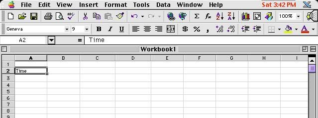
Fig 2 - entering text
Other text that we need can also be
entered, as shown in Fig 3. I have made a separate column for the
four different categories of data that we will need for each iteration:
the current time (t), the current position (q),
the current velocity (q'), and the current
acceleration (q''). In addition,
I have created a special section for the constants of the problem, namely,
the time step (Dt) which we will be using,
and the quantity g/L which we will need shortly.
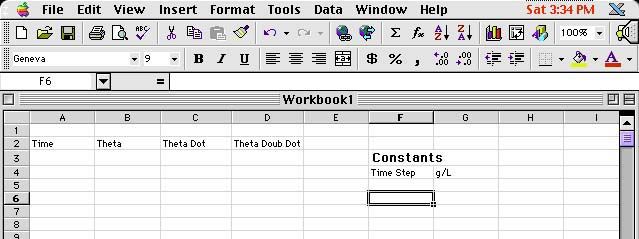
Fig 3 - more text
Next, we proceed to enter the known initial conditions for time t=0. Since we want to model the swinging pendulum experiment that we did in Kunkle Lounge, we put the initial position to some value (this really is up to you to decide what to put here, but for this example you might want to work along with me and use the same numbers I do. You can always change them later - after all, they are just numeric data!) I choose the initial position as 0.5, the initial velocity as 0, the time step as 0.1, and g/L as 1. Putting in everything we know, we get the following picture (Fig 4). Notice that text data is justified to the left of the cell, and numeric data to the right of the cell. This is just a convention that helps to distinguish between the two.
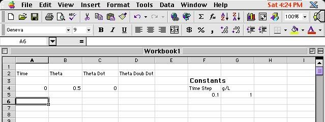
Fig 4 - numeric data
Ok, now comes the hard part:
formulas. Since we have exhausted all the known data of our problem,
we now have to use other facets of our problem to fill in the blanks.
What about the acceleration at t=0? Is there an equation that we
have for that? Check back above in case you forgot.
Knowing that we can relate the acceleration
and position of the pendulum at any instant in time through the governing
equation, we now need to let the spreadsheet know about this equation.
First, place your cursor over the cell for the acceleration at t=0 and
click. See figure 5:
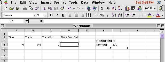
Fig 5 - the beginning of a function
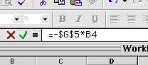
Next, in order to denote that we are entering an equation, type an equals sign (=) into the special cell that lies above the top row and under the toolbar. (Note: you can also just click on the equals sign that is right there). Now, type in the equation - since we know that the acceleration is given by -(g/L)*q we tell the spreadsheet to multiply the value found in the G4 cell by the value found in the B4 cell. In addition to this, we need to make sure the spreadsheet understands that the quantity (g/L) will always be found in the G4 cell, so we denote this type of absolute reference by preceding each character by a "string" marker ($). Now, if we paste the function somewhere else, the reference to cell G5 won't change to G6, etc. but will always be the same. But, since the value of theta found in cell B4 is only good for the first time step, we don't want that reference to stay constant, so we don't include the $ markers for it. The final equation will look like Fig 6. Hit the return key to enter it in.
 |
 |
| Fig 6 - the completed function and ... | Fig 7 - the result |
Ok, now we have filled in completely the t=0 line, so it's time to move on, literally. We first need to define the next time interval. Do this by entering a formula for the time t=1. Add the value of Dt to the value of t in the cell directly above it. Don't just type in the number .001, but instead reference the cell where Dt is located, that way if you want to change Dt later on all you'll have to do is change one cell and all the rest will automatically update themselves. Don't forget to make it an absolute reference! When you are done, your equation should look like: =A4+$F$5 The value of .001 should appear in the cell as expected.
Now, finally, we get to put old Euler to work: If you don't remember how to get the next value of the position in time, refresh your memory by looking back above. The equation you enter into the B5 cell should look like: =B4+C4*(A5-A4) Why? Next, using the same approximation, move on to the B6 cell and enter the correct equation for the value of the velocity. The answer it produces when you hit the enter key should be -.05 Now for the last cell in the time step t=1. Since we have already typed in the formula which relates the acceleration to the position of the pendulum at any instant, all that we need do is copy the equation from the t=0 cell to the t=1 cell. Do this by first highlighting the D4 cell and the D5 cell simultaneously (ie: hold down the button while moving the mouse over both of them) Then either click on the Edit->Paste Down menu or just type in Control-D and the formula will automatically copy itself into the D5 cell. Compare the two equations in the D4 and D5 cell. Why did some of the numbers change, and some did not?
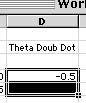
Fig 8 - copying an equation
Whew! we have finally typed in all the equations we need. Now it's time to iterate! But before you do that, it is probably a good idea to save your work. Next, highlight all four cells in the t=1 row only. Then, like before, drag down to paste the formulas down. Note that if you click and drag the lower right corner of the cell (where the little fancy square is) the spreadsheet will automatically copy everything for you. You are integrating forward in time! For a start, I copied down to the 210th cell.
![]()
The Excel Spreadsheet - Plotting the Results
Ok, now that we have solved the equation numerically, how do we visualize the results? Obviously we need to make some sort of plot. Do this easily by clicking on the "B" button, which highlights the whole B column (See Fig 9).
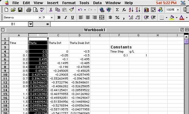
Fig 9 - making a chart
Then, go up and click on the chart button on the toolbar. Select the type of chart you want (I chose a line chart). You can click on the sample button to get an idea of what the chart will look like. When you are satisfied, click on the "finish" button, and there you go. You can drag the chart wherever you want to put it. Hopefully you got something like Fig 10. Notice that the horizontal axis is the row number of the cell that each data point comes from. You can have fun and double click all over the chart to bring up menus that allow you to change the color, labels, x-axis data, etc - but I just left it plain Jane.
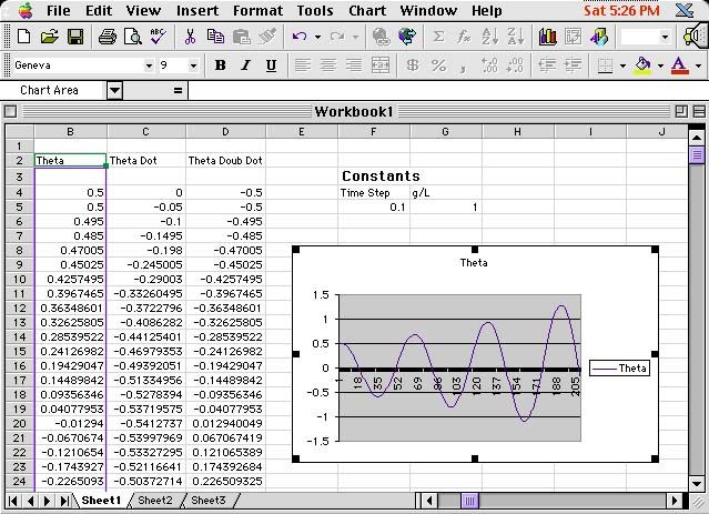
Fig 10 - the chart
![]()
Interpreting the Results
Ok, now for the fun part - where you can ask yourself the question, "What does it all mean?" The first thing that you should notice (knowing from class that the correct solution to the DE is a cosine function of constant amplitude) is that the amplitude seems to be getting very large, very fast. In fact, we started out with an amplitude of 0.5 and after 20s we have an amplitude of over twice as large! Of course one interpretation of this phenomena is that we discovered a perpetual motion machine (or perhaps people walking on the overhead bridges in Kunkle were adding energy to our system). On the more cautious side, the other possibility is that our solution is not very accurate. After all, 0.1s is kind of a big value for Dt.
To improve the accuracy of the solution, we need to make Dt smaller. Since we were foresighted enough to make an absolute reference to the one cell containing the time step information, all we need to is change the value in the F5 cell to something smaller, and the rest will take care of itself. I chose to change the time step to 0.01.
Notice that the chart also changed, but this time we don't get to see much happening, because now we are only seeing about 2s worth of oscillation. The solution to this? Just go down to the bottom row of your cells, and integrate forward some more in time. I went a bit further this time and dragged the corner down to the 3000th cell. Also, you will need to change the range on your graph so that it reads all the way down there. Do this by clicking on the chart (so that it is outlined in little black boxes) and then click on the chart->source data menu. Change the line that says: Sheet1!$B$2:$B$210 to: Sheet1!$B$2:$B$3000 This will instruct the chart to read all the data. How does the amplitude change with time now? You may want to save your graphs using different time steps, for later comparison.
![]()
Measuring the Period of Oscillation
Now, to complete the assignment, we
need to measure the period of the oscillation. There are a few ways
that you could do this, so if you have an idea - then try it out!
The way I'm going to present is only one way out of many. You can
check your final answer with mine though if you like.
First, I created four more text cells
in a row, with their corresponding data cells right below them. (see
Fig 11) To measure the period we need to know the number of time
steps traversed between two points on the graph of the same phase.
Since our oscillation started out at max amplitude, I first called a function
that finds the maximum value in the B column. Since the amplitude
is still increasing a little each time, the =MAX(B4:B2760) function will
pick out the value of the last amplitude peak on the graph. I put
this function in the F23 cell. Then I employed a function in the
G23 cell which was: =MATCH(F23,B4:B2760,0). The match function
returns the row number of the cell which has the value found in F23, namely
the max value! That way, I then know the time interval during which
the last peak in amplitude occurs. You can look up help on these
functions and more through the online help. In the third cell,
I put a space for how many peaks occurred in the graph. I just had
to enter this number visually each time the graph changed. Finally,
in the fourth cell, I entered the equation: =(G23-4)*F5/H23
so that I would get the period - total time traversed divided by the number
of wavelengths traversed. I had four peaks, and so my measured period
turned out to be 6.2775.
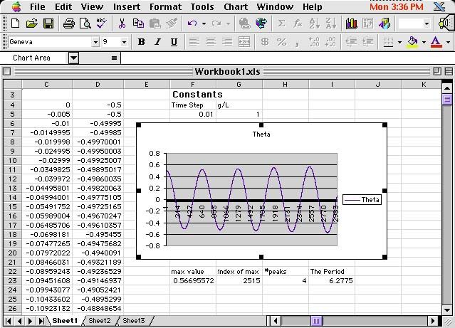
Fig 11 - the completed worksheet
Since we solved this DE exactly
in class, we know what the actual period should be: the formula
for the period is: P=2p/w
And the formula for the angular frequency is root(g/L).
Therefore, for my value of g/L of 1.0, the period should be around 6.2832.
A few notes on this method. If your initial value for the velocity is anything but zero, you will have to put in another function that finds the first maximum value on the graph since t=0 won't be at the maximum aplitude anymore. Just remember that you need to get two points of exactly the same phase. If you want to change the time step and number of cells integrated you must change the following: index of chart data, index of max value function, index of match function, #of peaks observed cell. Of course, your error of the period you get will depend strongly on how large your time step is, and how far you integrated in time. You will also will want to measure the period for different amplitudes, which is now easy to do - just change the initial conditions. Have fun!
![]()
Coming in the future (possibly): More sophisticated integration routines: Modified Euler's Method, and more. . .
![]()
![]() Please
email us with your response to this tutorial! Did you find it helpful,
insightful, boring, a waste of your time? Did you think this tutorial
was more or less helpful than the book and/or lecture in aiding you to
complete the spreadsheet assignment?
Please
email us with your response to this tutorial! Did you find it helpful,
insightful, boring, a waste of your time? Did you think this tutorial
was more or less helpful than the book and/or lecture in aiding you to
complete the spreadsheet assignment?
![]() Prepared
by Mike Stubna and Wendy McCullough.
Prepared
by Mike Stubna and Wendy McCullough.
This page was last modified on .
© Copyright 1999 by Mike Stubna, Wendy McCullough and Gary L. Gray. All rights reserved.